Linear Regression

Regression is an fairly important concept in data analysis as it shows potential trends in data. Its seems like a fun exercise to create my own algorithm to generate a regression line from a set of data points, so that's what I'll be doing today.

Setup

Here's the code I used to generate some test data and draw the regression line.

import math  
import random  
import numpy as np  
import matplotlib.pyplot as plt  
  
random.seed(0)  
  
minimum = 1  
maximum = 10  
points = 10  
  
x = [0] * points  
y = [0] * points  
  
def populate_randomly(x, y, length):  
    for i in range(length):  
        x[i] = random.randint(minimum, maximum)  
        y[i] = random.randint(minimum, maximum)  
  
populate_randomly(x, y, points)  
  
a = 1  
b = 0  
  
def apply_function(x, a, b):  
    return a * x + b  
  
def apply_regression(a, b, array):  
    for i in range(len(array)):  
        array[i] = apply_function(array[i], a, b) 
  
  
line_x = np.linspace(minimum, maximum, (maximum - minimum) * 2)  
line_y = line_x.copy()  
apply_regression(a, b, line_y)  
  
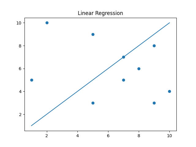
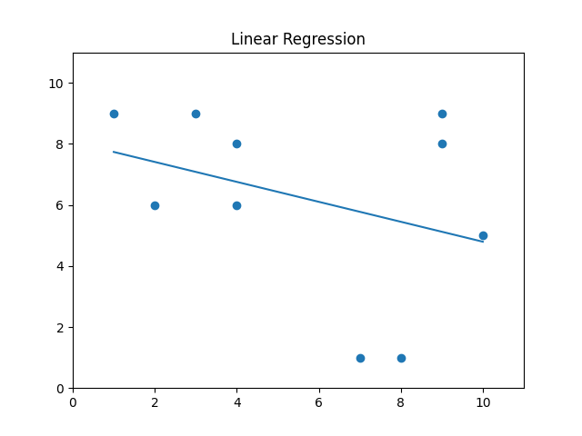
plt.scatter(x, y)  
plt.plot(line_x, line_y)  
plt.title("Linear Regression")  
plt.show()

I'm setting the random seed while I create my function, but when I'll try other random datasets and datasets with actual correlation after I'm done.

This is what the visualization looks like:

The slope and intercept

Now the actual problem is how I'm going to set the values of $a$ and $b$, which are the slope and intercept of the line respectively.

I know from statistics that Linear regression lines are created from minimizing the sum of squared error (SSE) from the line to the data points. Here's my function to calculate SSE:

def SSE(a, b, x, y):  
    sse = 0  
    for i in range(len(x)):  
        sse += (apply_function(x[i], a, b) - y[i]) ** 2  
    return sse

From just messing around around with the values of $a$ and $b$, and just from reasoning, I see that the slope and intercept values that minimize the SSE depend on each other, meaning that I can't just find the optimal slope then the optimal intercept, as the optimal slope depends on what the intercept is and vice versa.

Shown below is a 3D Plot I created to illustrate this

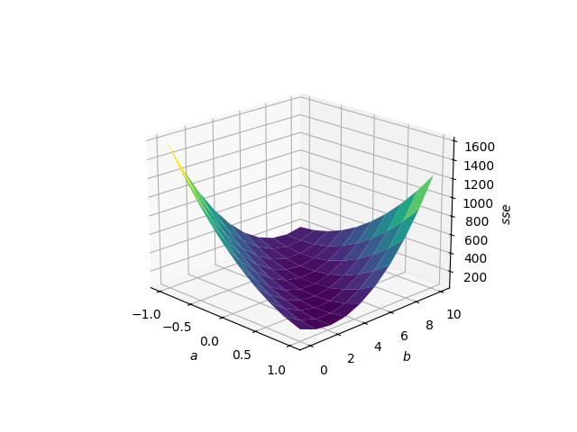
So I have to find the minimum value of this surface, which would be trivial if I had a closed form expression for the surface, but unfortunately I do not.

Finding the minimum

Looking surface above, I do have an idea though. I can start at any point $(a,b)$ and then sample points that are all an equal distance from this point and pick the direction that results in the greatest drop in SSE. Then, travelling in that direction until the minimum is found should result in the smallest possible SSE.

Just to see if this Idea works, I'm going make a steepest descent function that checks 360 degrees of rotation like so:

def steepestDescent(a, b, x, y):  
    min_a = a  
    min_b = b  
    minSSE = SSE(a, b, x, y)  
    for i in range(359):  
        a1 = a + math.cos(i * math.pi / 180)  
        b1 = b + math.sin(i * math.pi / 180)  
        sse = SSE(a1, b1, x, y)  
        if sse < minSSE:  
            minSSE = sse  
            min_a = a1  
            min_b = b1  
    return min_a, min_b

And then test it with an arbitrary number of iterations to see how close it gets to the real values

# Actual Values of a & b that minimize SSE
# a = -0.267966  
# b = 7.68819    
  
a = 0
b = 0

for i in range(10):  
    a, b = steepestDescent(a, b, x, y)  
  
print("a: " + str(a) + " b: " + str(b))

And the output of this code is...

a: -0.2719943210376332 b: 7.730975310123672

Creating a plot that looks like:

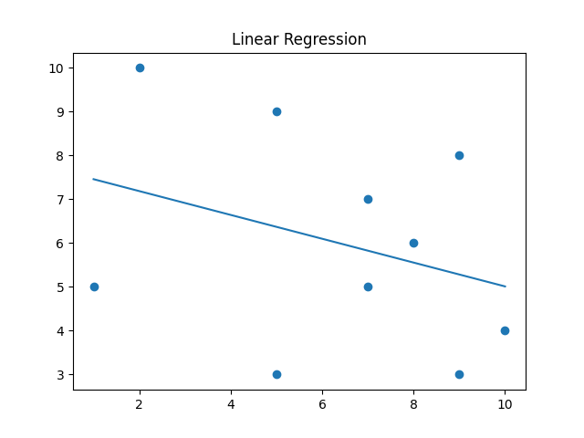
I think that's pretty good for me just guessing the number of iterations. So now to get this closer to actual minimization there is a few things to do. I need to figure out how many angles to check, how many iterations to run, and what I think will be most difficult: the distance to check the steepest descent in, as I'm currently just checking the unit circle.

Optimization and Improvement

The first thing I'll do is decouple the distance for the angle check from the distance traveled. I'll set the distance checked by the angle to be arbitrarily small, and the distance travelled will be set such that the SSE is minimized.

Here are the function's that does this

# Made for simplification
def travel(a, b, distance, angle):  
    if angle == -1:  
        return a, b  
    return a + distance * math.cos(angle), b + distance * math.sin(angle)
      
# Changes steepestDescent() to just return the angle
def findAngle(a, b, x, y, distance, angles):  
    min_angle = -1  
    minSSE = SSE(a, b, x, y)  
    for i in range(angles - 1):  
        a1, b1 = travel(a, b, distance, i * 2 * math.pi / angles)  
        sse = SSE(a1, b1, x, y)  
        if sse < minSSE:  
            minSSE = sse  
            min_angle = i * 2 * math.pi / angles  
    return min_angle  
    
# Finds the distance that minimizes SSE by using the positive concavity of the function to find a minimum within a certain threshold
def findDistance(a, b, x, y, angle, startingDistance, increment):  
    if angle == -1:  
        return 0  
  
    d = startingDistance  
  
    while True:  
        a1, b1 = travel(a, b, d, angle)  
        v1 = SSE(a1, b1, x, y)  
  
        a2, b2 = travel(a, b, d + increment, angle)  
        v2 = SSE(a2, b2, x, y)  
  
        a3, b3 = travel(a, b, d + 2 * increment, angle)  
        v3 = SSE(a3, b3, x, y)  
  
        if v2 > v1 or v3 > v2:  
            if math.fabs(v3 - v1) < 10 ** -10:  
                return d + increment  
            else:  
                return findDistance(a, b, x, y, angle, d, increment / 2)  
        d += increment

The distance function uses a margin of error of $10^{-10}$ to find the minimum on the angle.

This loop then iterates until the angle function indicates that the point has been minimized:

while angle != -1:  
    angle = findAngle(a, b, x, y, 10 ** -5, 10 ** 3)  
    distance = findDistance(a, b, x, y, angle, 0,10 ** 3)  
    a, b = travel(a, b, distance, angle)

The angle function checks $10^{3}$ angles a distance of $10^{-5}$ away to best mimic the gradient of the function, and the distance function starts with an increment of $10^{3}$ before lowering that to find a more precise minimum.

When there are more points in a dataset, the accuracy will need to be more seriously considered as the SSE calculations, which there are a lot of especially with the high number of angles checked, will become more computationally expensive.

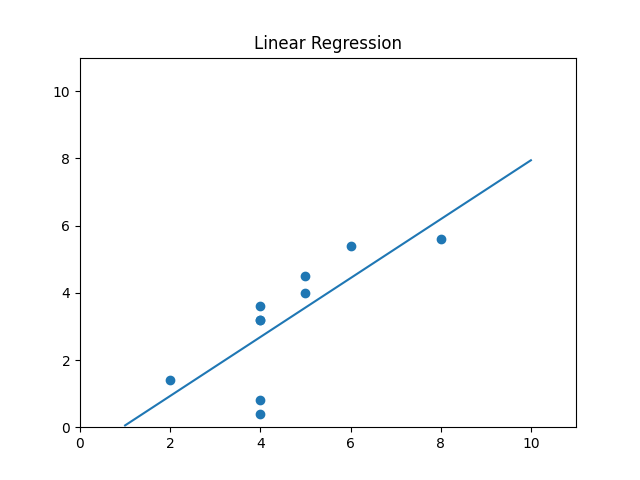
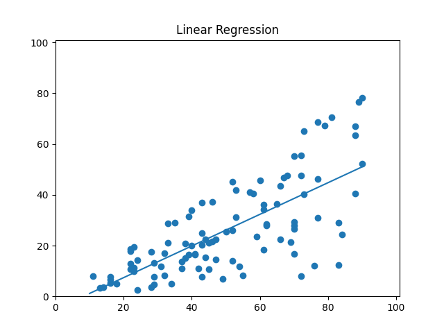
Many of these values are chosen arbitrarily but the code runs fairly quickly and the output is much more accurate at a: -0.2679657464848839 b: 7.688184072259003 so I'll call that a success.

Here's some more examples of the linear regression working

Wrapping Up

I think this is a fun example of using a mathematical abstraction to solve a problem. I wasn't expecting Calc 3 to make an appearance here but I'm glad it did.

Check out the source code